Worked Example — MLB Home Runs

Step 1 of 8

The raw data

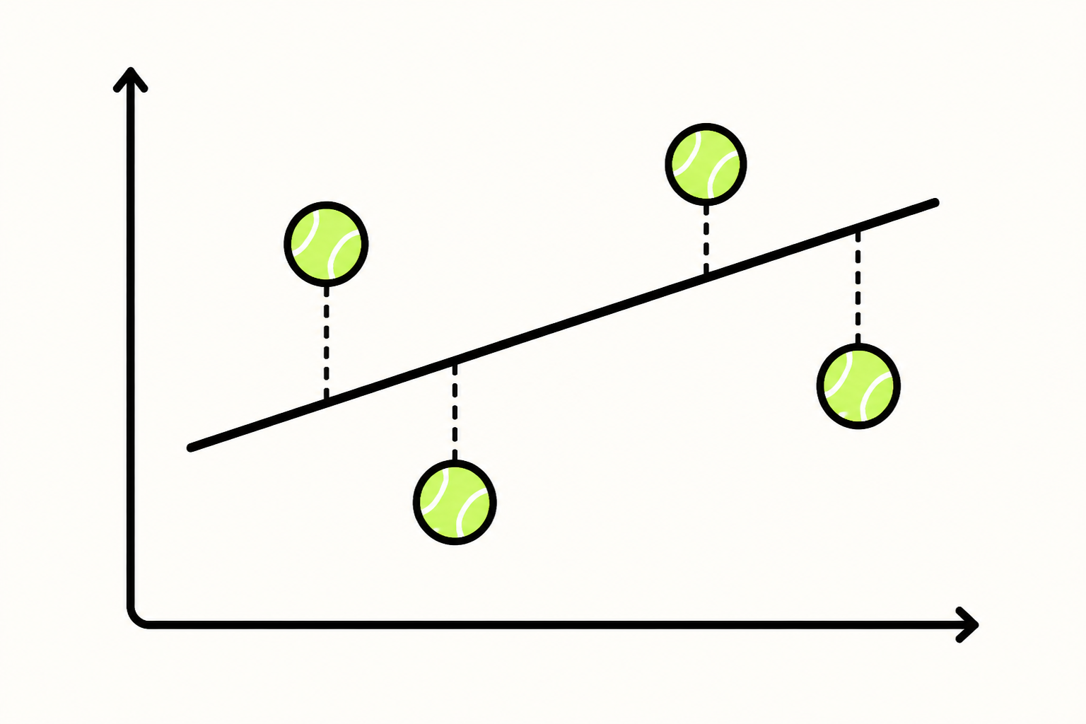
Do teams that hit more home runs score more runs? x = home runs, y = runs scored — both per season, six teams.

Six rows, two columns

6 MLB teams — one season

Team	Home runs (x)	Runs scored (y)
Yankees	245	807
Dodgers	221	758
Red Sox	198	726
Astros	214	749
Cubs	177	691
Padres	162	668

Moneyball connection Billy Beane's A's found that some cheap counting stats had a big effect on winning. Spotting which x-variables move y the most is exactly what regression does.

Step 2 of 8

Find the means x̄ and ȳ

The means are the data's centre of gravity. A key OLS fact: the fitted line always passes through the point (x̄, ȳ).

Crosshair marking the mean point of a scatter

The line must pass through (x̄, ȳ)

x̄ — mean home runs

x̄ = (245 + 221 + 198 + 214 + 177 + 162) / 6 = 1217 / 6 = 202.83

ȳ — mean runs scored

ȳ = (807 + 758 + 726 + 749 + 691 + 668) / 6 = 4399 / 6 = 733.17

(x̄, ȳ) = (202.83, 733.17) is the "average team" in this sample. No matter what the slope and intercept turn out to be, the regression line is guaranteed to run through this point.

Step 3 of 8

Compute Sxx and Sxy

Sxx measures how spread out the home-run counts are. Sxy measures how x and y move together. Both feed straight into the slope.

Arrows showing deviations from the centre line

Deviations from the mean

Deviation table

Team	xᵢ−x̄	yᵢ−ȳ	(xᵢ−x̄)²	(xᵢ−x̄)(yᵢ−ȳ)
Yankees	42.17	73.83	1778.3	3113.7
Dodgers	18.17	24.83	330.1	451.2
Red Sox	−4.83	−7.17	23.3	34.6
Astros	11.17	15.83	124.8	176.8
Cubs	−25.83	−42.17	667.4	1089.3
Padres	−40.83	−65.17	1667.1	2661.6
Σ	≈ 0	≈ 0	4591.0	7527.2

Sxx = Σ(xᵢ−x̄)²4591.0

Sxy = Σ(xᵢ−x̄)(yᵢ−ȳ)7527.2

The deviation columns sum to ≈ 0 — always true, and a handy arithmetic check. Sxy is large and positive: more home runs clearly travels with more runs.

Step 4 of 8

The slope β̂₁ and intercept β̂₀

With Sxx and Sxy in hand, the line is one division and one subtraction away.

Slope = rise ÷ run

Slope

β̂₁ = Sxy / Sxx = 7527.2 / 4591.0 = 1.639

Each extra home run is worth about 1.639 more runs.

Intercept

β̂₀ = ȳ − β̂₁ × x̄ = 733.17 − 1.639 × 202.83 = 400.73

ŷ = 400.73 + 1.639 × x

Matrix connection β̂₁ = Sxy / Sxx is exactly what β̂ = (XᵀX)⁻¹XᵀY gives for one predictor. Add more predictors and you need the full matrix; with a single x it collapses to this ratio.

Step 5 of 8

Fitted values ŷᵢ and residuals eᵢ

Plug each xᵢ into the line to get ŷᵢ. The residual eᵢ = yᵢ − ŷᵢ is how far off the model is for that team.

Scatter points with dashed lines to a fitted line

Each dashed gap is a residual

ŷᵢ = 400.73 + 1.639 × xᵢ

Team	yᵢ	ŷᵢ	eᵢ	eᵢ²
Yankees	807	802.3	+4.7	22.1
Dodgers	758	763.0	−5.0	25.0
Red Sox	726	725.2	+0.8	0.64
Astros	749	751.5	−2.5	6.25
Cubs	691	690.8	+0.2	0.04
Padres	668	666.2	+1.8	3.24
Σ			≈ 0	57.3

Residuals always sum to zero in OLS. The Astros' −2.5 means they scored 2.5 fewer runs than predicted — home runs alone can't capture everything (a few stranded runners, say).

Step 6 of 8

SSE and the variance estimate s²

SSE is the total squared error after fitting. s² estimates σ² — the natural scatter around the true line.

A residual gap drawn as a literal square

Square each residual, then add

Sum of squared errors

SSE = Σ eᵢ² = 22.1 + 25.0 + 0.64 + 6.25 + 0.04 + 3.24 = 57.3

Variance estimate

s² = SSE / (n − 2) = 57.3 / 4 = 14.33 s = √14.33 = 3.79 runs

Why n − 2? We used up 2 degrees of freedom estimating β̂₀ and β̂₁, so we divide by n − 2, not n. Writing n here is the most common slip on this topic.

Step 7 of 8

R² — how much we explained

R² answers: what proportion of the total variation in runs does the model account for?

A donut chart showing explained versus unexplained variation

Explained vs unexplained

Total sum of squares

TSS = Σ(yᵢ − ȳ)² = 5452.8 + 615.7 + 51.4 + 250.7 + 1778.3 + 4247.1 = 12396.0

R²

R² = 1 − SSE / TSS = 1 − 57.3 / 12396.0 = 0.9954

TSS (total)12396

SSE (unexplained)57.3

R²0.995

Home runs explain 99.5% of the variation in runs scored across these six teams. The other 0.5% is everything else — walks, singles, stolen bases. (Real research rarely gets this high; here it's genuine, since HR teams simply score more.)

Step 8 of 8

Putting it into words

Every quantity, its value, and what it actually means — plus how to phrase it in an exam.

A lightbulb representing the interpretation

From numbers to meaning

Summary

Quantity	Value	Meaning
β̂₁	1.639	+1 HR → +1.639 runs
β̂₀	400.73	Baseline runs at x = 0
SSE	57.3	Unexplained squared error
s	3.79	Typical miss (± runs)
R²	0.9954	99.5% of variation explained

How to write it in an exam

Slope: For each additional home run in a season, a team is estimated to score 1.639 more runs on average.

Intercept: A team hitting zero home runs is predicted to score 400.73 runs (non-HR scoring) — but x = 0 is outside the data, so it isn't practically meaningful.

R²: Home runs explain 99.5% of the variation in runs scored — an excellent fit.

Test yourself →