Worked Example — Runs from HR + Walks

Step 1 of 9

The raw data

Do runs depend on home runs and walks together? x1 = home runs, x2 = walks, y = runs. We use six familiar MLB clubs as a compact teaching sample.

Two predictors, one outcome

Six teams

Team	HR (x?)	Walks (x₂)	Runs (y)
Yankees	245	520	690
Dodgers	221	540	696
Red Sox	198	505	652
Astros	214	560	706
Cubs	177	480	623
Padres	162	500	632

Why two predictors?The Yankees mash home runs; the Astros draw walks to load the bases. Each stat captures scoring the other misses — exactly when reaching for a second predictor pays off.

Step 2 of 9

The model — from a line to a plane

One predictor drew a line. Two predictors draw a tilted sheet. Here's how to actually picture that.

Two dials feeding one reading

y = β₀ + β₁·x? + β₂·x₂ + ε

Picture it on the field

In Chapter 1 you drew a line on a flat graph: home runs along the bottom, runs up the side. Two directions — a 2-D picture.

Add walks and you need a third direction. Picture the outfield as a flat grid: home runs running out to centre field, walks running foul-line to foul-line. Every spot on that grid is one (HR, walks) combination, and the model floats a predicted runs value above it like a height. Join those heights up and you get a flat, tilted sheet hovering over the field — a plane.

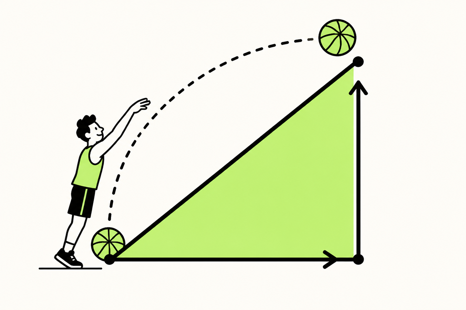
What each β does

β₁ is how steeply the sheet rises as you walk in the home-run direction; β₂ how steeply it rises in the walks direction; β₀ is the sheet's height above the corner where both are zero — the same "anchor" the intercept played in Chapter 1, and just as theoretical (no club hits 0 home runs and draws 0 walks).

And three or more predictors?Add a third stat — say stolen bases — and you'd need a fourth direction, more than anyone can draw. Mathematicians call that surface a hyperplane: literally "a plane in more dimensions." You can't picture a 4-D stadium, and you don't have to — the formula treats 2, 3 or 30 predictors identically. Here, "dimension" just means "one more thing you're measuring."

Step 3 of 9

What's a matrix? (and transpose)

Two new words before the formula — both simpler than they look.

1s · HR · walks

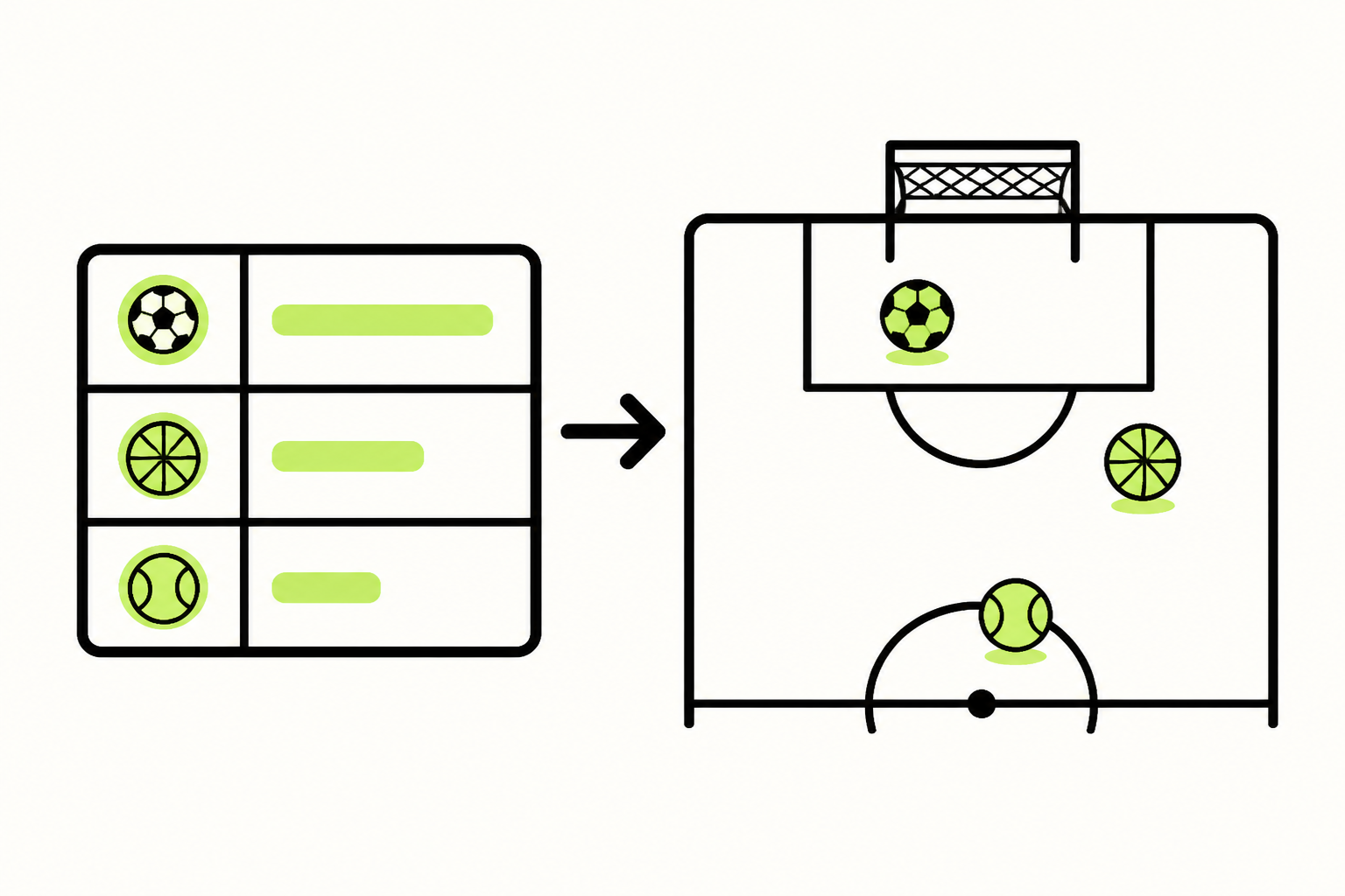
A matrix is just a table of numbers

You've read them all chapter. We stack our data into the design matrix X — one row per team, columns for [1, HR, walks] — and the runs into a column y.

1 HR walks Yk ⎡ 1 245 520 ⎤ ⎡ 690 ⎤ Dg ⎢ 1 221 540 ⎥ ⎢ 696 ⎥ Rs ⎢ 1 198 505 ⎥ y = ⎢ 652 ⎥ As ⎢ 1 214 560 ⎥ ⎢ 706 ⎥ Cb ⎢ 1 177 480 ⎥ ⎢ 623 ⎥ Pd ⎣ 1 162 500 ⎦ ⎣ 632 ⎦

That leading column of 1s is a bookkeeping trick — it lets the intercept β₀ fall out of the same formula as the slopes.

Transpose: tip the table on its side

The little ᵀ in Xᵀ means transpose: flip the table so every row becomes a column. Take just the first three teams:

X (rows = teams) Xᵀ (flipped) ⎡ 1 245 ⎤ Yankees ⎡ 1 1 1 ⎤ ⎢ 1 221 ⎥ Dodgers ⎣ 245 221 198 ⎦ ⎣ 1 198 ⎦ Red Sox

The first row of X, (1, 245), became the first column of Xᵀ. That's the whole operation — the table simply tips onto its side, so each variable ends up on its own row.

Why flip it?Lining the table up against its flipped self (and against runs) is what lets us measure how the predictors vary and how they track scoring — all at once. The next step turns that into the coefficients.

Step 4 of 9

The formula, piece by piece

It looks scary. It's really just Chapter 1's slope, written for more than one predictor.

Slopes ÷ spread

β̂ = (XᵀX)⁻¹ Xᵀy

Reading each piece in plain English

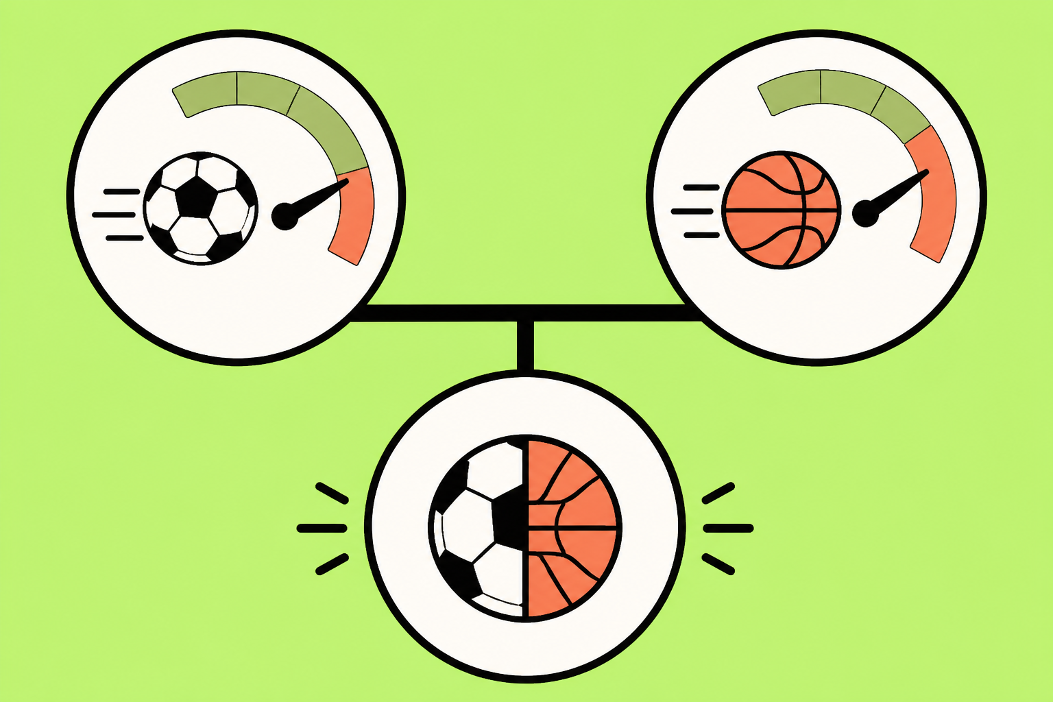
Xᵀy — pairs each predictor with runs: how strongly do home runs, and walks, each track scoring across the teams? (This is Chapter 1's Sxy.)

XᵀX — the flipped table times the original: how much do the predictors spread out and overlap? (Chapter 1's Sxx, now a small grid that also notices when HR and walks move together.)

( )⁻¹ — the inverse, which is the matrix version of dividing.

It's just Sxy / Sxx, grown upPut the pieces together and β̂ = (XᵀX)⁻¹Xᵀy reads as (how the predictors track runs) ÷ (how the predictors spread and overlap) — the exact multi-variable cousin of Chapter 1's slope = Sxy / Sxx.

The one genuinely hard bitInverting that 3×3 grid by hand is a slog, so we let R do it. The formula is what you carry forward — it works the same for one predictor or fifty.

Step 5 of 9

The coefficients

Solving the formula hands back all three numbers at once.

Three numbers define the plane

β̂₀ = 139.68 (intercept) β̂₁ = 0.508 (home runs) β̂₂ = 0.819 (walks)

ŷ = 139.68 + 0.508·HR + 0.819·walks

Both predictor coefficients are positive — more home runs and more walks each go with more runs. The intercept (139.68) is theoretical, as flagged in Step 2.

Step 6 of 9

Interpret — "holding the other constant"

The one genuinely new reading skill. Each coefficient is read with the other predictor frozen.

Vary one, freeze the other

β̂₁ = 0.508: among teams with the same number of walks, each extra home run is worth about 0.51 more runs on average.

β̂₂ = 0.819: among teams with the same number of home runs, each extra walk is worth about 0.82 more runs on average.

Why it mattersIn Chapter 1, home runs' slope quietly soaked up some of walks' effect too. Holding walks constant strips that out — you get each variable's own contribution.

Step 7 of 9

R² and adjusted R²

R² still measures variation explained — but adding predictors always nudges it up, so we adjust.

Adjusted R² adds a penalty

R² = 1 − SSE/TSS = 1 − 8.07/6275.5 = 0.9987 adjusted R² = 1 − (1−R²)·(n−1)/(n−p−1) = 1 − (1−0.9987)·5/3 = 0.9979

R²0.999

adjusted R²0.998

n, predictors p6, 2

Use adjusted R² to compare modelsIt only rises if a new predictor earns its place. If R² jumps but adjusted R² doesn't, the extra variable is just fitting noise.

Step 8 of 9

Is the model useful? The F-test

The overall F-test asks one question: do the predictors, together, explain anything?

Explained vs leftover variation

H₀: β₁ = β₂ = 0 (neither predictor helps) F = MSR / MSE = 1164.7 on (2, 3) df p-value ≈ 0.00006 → reject H₀

F-test vs t-testsThe F-test judges all predictors at once ("is this model worth anything?"). Each coefficient's individual t-test judges that one predictor on its own. In SLR they were the same; here they answer different questions.

Step 9 of 9

Predict & write it up

Plug new values into the fitted plane, then state the findings cleanly.

From plane to plain English

A team with 200 HR and 520 walks: ŷ = 139.68 + 0.508×200 + 0.819×520 = 667 runs

How to write it in an exam

Slopes: Holding walks fixed, each home run adds ≈0.51 runs; holding home runs fixed, each walk adds ≈0.82 runs.

Fit: The two predictors explain 99.9% of the variation in runs (adjusted R² = 0.998).

Overall: The F-test (F = 1164.7, p ≈ 0) shows the model as a whole is highly significant.

Test yourself →